Network/Graph Theory#
The basic unit here is called a Node (or a Vertex; ‘\(V\)’) and the link connecting two nodes/vertices is called an Edge (’\(E\)’). A map of these nodes and edges is a Network (or a Graph). To study a system or interactions therein, one may use analyses and models of Network theory, or Graph theory. This theory can act as a good tool for systems-level analyses, given that…
… one can cleanly define basic units in the system being study, in the form of Nodes.
… one can clearly define the nature of relations that connects these units, to delineate as Edges.
… one can infer organisational functionality or model development/evolution of the system based on the patterns of connectivity.
Resources:#
BCT stands for ‘Brain Connectivity Toolbox’. One can use the project bctpy for Python.
NetworkX is another Python library.
BRAPH: a brain analysis toolbox for graph theory.
Graph-Tool is also a python-based toolbox.
igraph is yet another graph-theoretic library for R and Python.
# Initialize Libraries
import numpy as np
import matplotlib.pyplot as plt
import bct as bct
import networkx as nx
Types of Network Models:#
Network models are generally represented in two forms. (1) edge-connectivity list, or edge-list, is generally a larger form of matrix (size \(V\times E\)) that defines which nodes are connected by a given edge. Whereas, (2) network-connectivity matrix may form a smaller matrix (of size \(V\times V\)), where each row and column represent a node and the value of the respective cell represents the presence/nature of the edge. For the rest of the notebook, one may assume that ‘connectivity matrix’, ‘adjacency matrix’, or ‘connectivity profile’ implies the network-connectivity matrix, unless otherwise specified. The networks can further be classified according to the properties of their connections:
Weighted v/s Binary edges: a network where a cell in the connectivity matrix is represented by a 0 implies absence of an edge. For binary networks like friendship/social networks or internet links, the 1’s represent the presence of an edge. For weighted networks like trust-based social networks or brain connectivity, the non-binary value represents the ‘weight’ or the strength of the connecting edge.
Directed v/s Undirected edges: while most networks we work with (concerning brain) may be undirected, there may be a directional value associated for other type of networks (for example, Markov chains). Undirected networks will always have symmetric matrices as their connectivity profile.
Signed v/s Unsigned networks: usually, a network will contain only positive values representing the strength/weight of the edges. However, in some cases (like coherence-based networks or correlation-networks), one may witness negative values and serve a functional use. As an example, one may use the signed edges to represent excitatory versus inhibitory neuronal connections.
Networks with Node Values: some networks may have nodes with values associated to them. These values may symbolise node strength, size of the region represented (for eg. ROI of the brain), or even the limit of connections that may exist (for eg. capacity of bus/train stations, airports, etc).
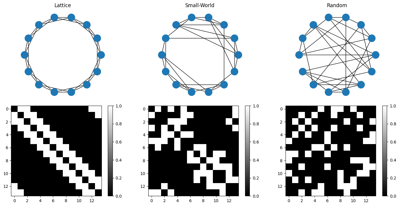
Network Structures and Small-worldness:#
Most common networks include the lattice (or regular) and random structures. A lattice/regular network has a proximity-based connectivity profile, that is, all nodes have similar or equal number of connections to the k-closest nodes. On the other hand, a random network will generally have a seemingly hap-hazard connectivity. According to Watts and Strogatz, 1998, real-world systems follow a principal of ‘Small-Worldness’, where even though the nodes have similar profiles of connectivity, occassionally one may find some random connections that account for ‘short-cuts’ across the network.

In the random network structure, an Erdös-Rényi Graph (ER Graph) is a special kind of graph where the random-rewiring maintains the over-all number of connections to a node. That is, if we start with a lattice structure where each node has k edges, then the randomized ER graph of that network will maintain that all nodes have k connections. This idea is very commonly used to generate null-graphs to assess the SNR of the salient connections.
n = 14; # Number of nodes in the network

# Make a Lattice:
adj_lattice = np.zeros((n,n));
for i in np.arange(n):
    for j in i+np.arange(3):
        if j<n: adj_lattice[i,j] = 1;
        else: adj_lattice[i,j-n] = 1;
adj_lattice += adj_lattice.T;
adj_lattice[np.arange(n),np.arange(n)] = 0;
del i,j;

# Small World Structure:
adj_smallworld = bct.latmio_und_connected(adj_lattice, itr=2)[1];

# Random Structure:
adj_random = bct.randmio_und(adj_lattice, itr=2)[0];

# Plot the Structures:
fig = plt.figure(figsize=(14,7));

ax11 = fig.add_subplot(231, aspect='equal');
nx.draw_circular(nx.Graph(adj_lattice));
plt.title('Lattice');

ax12 = fig.add_subplot(234, aspect='equal');
plt.imshow(adj_lattice, vmin=0, vmax=1, cmap='gray');
plt.colorbar();

ax21 = fig.add_subplot(232, aspect='equal');
nx.draw_circular(nx.Graph(adj_smallworld));
plt.title('Small-World');

ax22 = fig.add_subplot(235, aspect='equal');
plt.imshow(adj_smallworld, vmin=0, vmax=1, cmap='gray');
plt.colorbar();

ax31 = fig.add_subplot(233, aspect='equal');
nx.draw_circular(nx.Graph(adj_random));
plt.title('Random');

ax32 = fig.add_subplot(236, aspect='equal');
plt.imshow(adj_random, vmin=0, vmax=1, cmap='gray');
plt.colorbar();

fig.tight_layout(pad=1);
plt.show();
del fig, ax11, ax12, ax21, ax22, ax31, ax32;
Network Metrics:#
Node Degree or Node Strength: simply put the total amount of all connections to the node is termed as node strength. For binary networks, strength can be measured as the total number of connections to the node. For directed connections, the degree is divided into an In-Degree and an Out-Degree.
Path Length: path length is the shortest distance between two given nodes. Global and local structures may utilise the metric of ‘average path length’.
Efficiency: defined as the average of the inverse of path length, the global efficiency and local efficiency can be used to compare networks.
Centrality: If a node is connected in a manner that higher amount of information will pass through it than others, then the node is termed to be more ‘central’ to the structure. Depending on what kind of value is being passed, one may find different types of centrality measures.
The most common centrality measures are described here, but researchers have come up with other types of this metric as well. Betweenness Centrality of a node is the ratio of the shortest path from the node to every other node to the shortest pathlength. Degree Centrality of a node is the number of connections the node has. Closeness Centrality is the average path-length of the given node with all other nodes of the graph. Eigenvalue/Eigenvector Centrality is the eigenvector associated to the vector of nodes based on the connectivity profile of the network.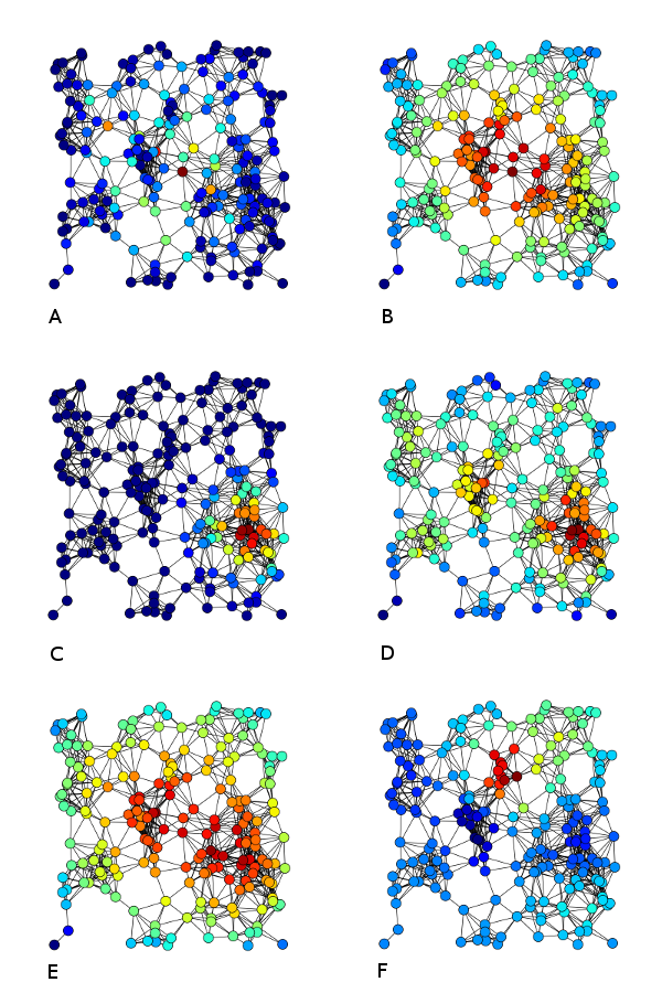
Figure Source:
Wikipedia article on ‘Centrality’; described as: Examples of A) Betweenness centrality, B) Closeness centrality, C) Eigenvector centrality, D) Degree centrality, E) Harmonic centrality and F) Katz centrality of the same graph.Diversity Coefficient: The Shannon-entropy based diversity coefficient measures the diversity of intermodular connections of individual nodes.
Flow Coefficient: similar to the Betweenness Centrality metric, flow measures the capacity of information flow through a given node. (source: Honey et.al., 2007, PNAS).
Reachability: this is a binary valued metric that tries to establish if a node can reach another node.
Rich Club Coefficient: rich clubs are established by establishing connectivity between nodes of degree k or higher. Rich club coefficient of a node at level k is the fraction of edges that connect nodes of degree k or higher out of the maximum number of edges that such nodes might share.
Some of the definitions were sourced from: BCT.
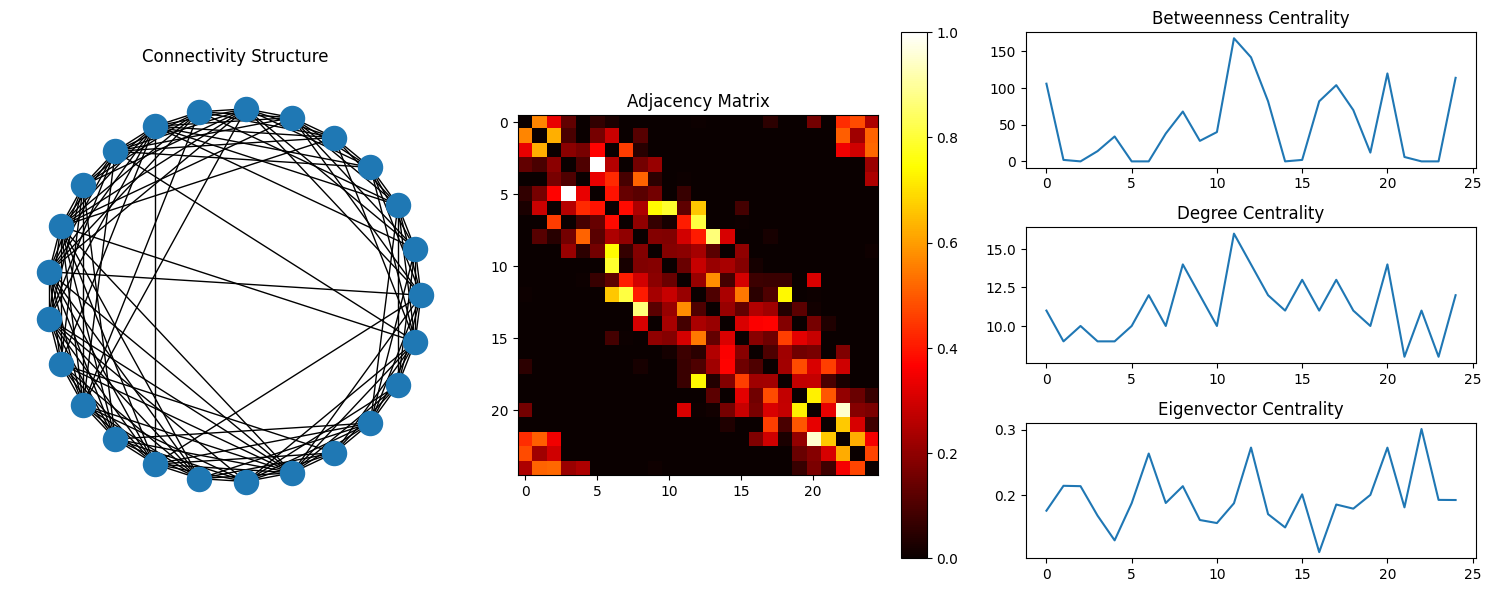
n = 25;

# Generate The Required Matrix
adj = np.random.normal(size=(n,n));
adj = (adj + adj.T)/np.max(adj);
adj[adj<0] = 0;
adj[np.arange(n),np.arange(n)] = 0;
adj = bct.latmio_und(adj, itr=np.random.choice(n))[1];

# Now let's try and plot some of the network metrics (per node)
adj_bet = bct.betweenness_wei(adj);            # Betweenness Centrality (for Weighted Networks)
adj_deg = bct.degrees_und(adj);                # Degree Centrality (for Undirected Networks)
adj_eig = bct.eigenvector_centrality_und(adj); # Eigenvector Centrality (for Undirected Networks)
# Plots:
fig = plt.figure(figsize=(15,6));
G = nx.Graph(adj);

ax1 = fig.add_subplot(131, aspect='equal');
nx.draw_circular(G);
plt.title('Connectivity Structure');

ax2 = fig.add_subplot(132);
plt.imshow(adj, vmin=0, vmax=1, cmap='hot');
plt.colorbar();
plt.title('Adjacency Matrix');

ax31 = fig.add_subplot(333);
plt.plot(adj_bet);
plt.title('Betweenness Centrality');

ax32 = fig.add_subplot(336);
plt.plot(adj_deg);
plt.title('Degree Centrality');

ax33 = fig.add_subplot(339);
plt.plot(adj_eig);
plt.title('Eigenvector Centrality');

fig.tight_layout(pad=1);
plt.show();
del fig, ax1, ax2;
Mesoscale Structures:#
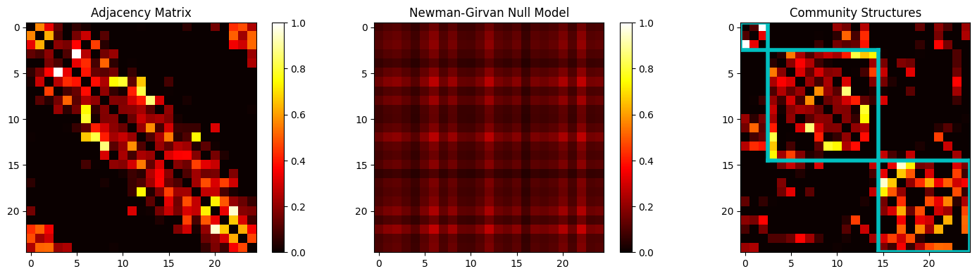
Community Structures – Modularity and Clustering:#
Modularity analysis is a very common theme to establish clusters of nodes that form strong interconnected structures within the network. One starts by solving for the modular communities using the formula:
Solving for modularity matrix requires one to use the optimum value of \(\gamma\) as a factor that regulates the null model of the connectivity matrix \(A_{ij}\), represented as \(P_{ij}\). One can use the Newman-Girvan null model which maintains the degree-distribution of a given network by substituting \(P_{ij} = \frac{k_i\cdot k_j}{2K}\) for binary models and \(P_{ij} = \frac{s_i\cdot s_j}{2W}\) for weighted ones. For the substitutions, \(k_i\) (or the weighted \(c_i\)) is the degree of \(i^{th}\) node, \(K\) is total number of connections in the binary network, and \(W = \frac{1}{2}\cdot\sum_{(i,j)}A_{ij}\) for weighted networks. Therefore, one must optimize the \(Q\)-parameter for either of these two cases:
From this optimized parameter, one can extract the matrices that may show one (or more often a combination) of the three basic structures:
Modular Community Structures form when the edges can be re-arranged to form groups that, when plotted, lie on the diagonal of the adjacency/connectivity matrix. These groups can easily be separated to form their own groups or ‘communities’.
Bipartite Structure forms when the edges can be re-arranged to diverge away from the diagonal of the matrix. When plotted, they appear as highlighted corners away from the diagonal.

Core-Periphery Structures form when the edges can be re-arranged to include some values close to the diagonal that extend all the way to the corners of the matrix. Unlike bipartite models, there is no lack of connectivity closer to the diagonal, but unlike the modular communities, connectivity doesn’t span the entire diagonal either.
# Using the Adjacency Matrix from earlier...
s = np.sum(adj, axis=0).reshape(-1,1);
m = np.sum(adj);        # w = np.sum(adj)/2; m = 2 * w;
adj_null = (s * s.T)/m; # Newman-Girvan Null Model = (s*s.T)/(2*w);


############################################################################
#
# One may go ahead and do the modularity optimization using their own code,
#  however, BCT has a functions for it:
#
############################################################################

M = np.arange(n); # initial community affiliations
Q0 = -1; Q1 = 0;  # initialize modularity values
while Q1-Q0>1e-5:
    Q0 = Q1; # perform community detection
    [M, Q1] = bct.community_louvain(adj, ci=M);
[xy_bounds, idx] = bct.grid_communities(M);
# Plot the Structures:
fig = plt.figure(figsize=(15,4));
G = nx.Graph(adj);

ax1 = fig.add_subplot(131);
plt.imshow(adj, vmin=0, vmax=1, cmap='hot');
plt.colorbar();
plt.title('Adjacency Matrix');

ax2 = fig.add_subplot(132);
plt.imshow(adj_null, vmin=0, vmax=1, cmap='hot');
plt.colorbar();
plt.title('Newman-Girvan Null Model');

ax3 = fig.add_subplot(133);
plt.imshow(adj[idx,:][:,idx], vmin=0, vmax=1, cmap='hot');
for i in np.arange(len(xy_bounds)-1):
    plt.plot([xy_bounds[i],xy_bounds[i]],[xy_bounds[i+1],xy_bounds[i]],'c',linewidth=4);
    plt.plot([xy_bounds[i+1],xy_bounds[i]],[xy_bounds[i],xy_bounds[i]],'c',linewidth=4);
    plt.plot([xy_bounds[i+1],xy_bounds[i]],[xy_bounds[i+1],xy_bounds[i+1]],'c',linewidth=4);
    plt.plot([xy_bounds[i+1],xy_bounds[i+1]],[xy_bounds[i],xy_bounds[i+1]],'c',linewidth=4);
plt.title('Community Structures');

fig.tight_layout(pad=1);
plt.show();
del fig, ax1, ax2;
Other Concepts:#
Some graph theoretical concepts were not covered. However, they are worth looking into! These topics include (but not limited to) network motifs, multilayered networks, dynamics and control of networks, generative models, and topological properties like holes and Rentian scaling.

References:#
Alon, U. Network motifs: theory and experimental approaches. Nat Rev Genet 8, 450–461 (2007). DOI: 10.1038/nrg2102
Calderer Genís, Kuijjer Marieke L., Community Detection in Large-Scale Bipartite Biological Networks, Frontiers in Genetics, vol. 12, 2021. DOI: 10.3389/fgene.2021.649440
Centeno, E.G.Z., Moreni, G., Vriend, C. et al. A hands-on tutorial on network and topological neuroscience. Brain Struct Funct 227, 741–762 (2022). DOI: 10.1007/s00429-021-02435-0
Elliott A, Chiu A, Bazzi M, Reinert G, Cucuringu M. (2020) Core–periphery structure in directed networks. Proc. R. Soc. A 476: 20190783. DOI: 10.1098/rspa.2019.0783
Honey CJ, Kötter R, Breakspear M, Sporns O (2007) Network structure of cerebral cortex shapes functional connectivity on multiple time scales. PNAS. DOI: 10.1073/pnas.0701519104
Lohse C, Bassett DS, Lim KO, Carlson JM (2014) Resolving Anatomical and Functional Structure in Human Brain Organization: Identifying Mesoscale Organization in Weighted Network Representations. PLoS Comput Biol 10(10): e1003712. DOI: 10.1371/journal.pcbi.1003712
Megan M. Sperry, Qawi K. Telesford, Florian Klimm, Danielle S. Bassett (2017) Rentian scaling for the measurement of optimal embedding of complex networks into physical space, Journal of Complex Networks, Volume 5, Issue 2, June 2017, Pages 199–218, DOI: 10.1093/comnet/cnw010
Mikail Rubinov, Olaf Sporns. Complex network measures of brain connectivity: Uses and interpretations, NeuroImage. Volume 52, Issue 3, 2010, Pages 1059-1069, ISSN 1053-8119. DOI: 10.1016/j.neuroimage.2009.10.003
Sporns O, Honey CJ, Ko¨tter R (2007) Identification and Classification of Hubs in Brain Networks. PLoS ONE 2(10): e1049. DOI: 10.1371/journal.pone.0001049
Tunç B, Verma R (2015) Unifying Inference of Meso-Scale Structures in Networks. PLOS ONE 10(11): e0143133. DOI: 10.1371/journal.pone.0143133