Networks in Social Media

Networks in Social Media#

The key benefit of this approach is that it affords the flexibility to study social networks by moving beyond the number of interactions people have to considering textual content, timing, and context, ultimately making use of the rich data provided from social media. [1]

Entropy-based Classification of Retweeting Activity on Twitter (Ghosh et al., 2011)[5]#

As for a specific example of how information-theoretic concepts have been successfully applied to characterize processes in social networks and social media, we can look to Ghosh et al., 2011 [5]. In their work, they sought to automatically classify different types of activity on Twitter. They had a particular interest in differentiating between retweet activity that was spam-like (e.g., a bot account that repeatedly retweets a singular tweet) vs. successful information dissemination.
This might conceptually relate to the concept of mutual information, whereby in characterizing retweet activity and content, you are ultimately trying to see how much the retweet content actually gives any information about what the original tweet was. In other words, bot accounts spam-retweeting isn’t particularly informative in studying actual Twitter user behavior and information propagation.
Problem statement: manual analysis of retweeting activity is labor-intensive. Given some user-generated content or tweet, Ghosh et al. aimed to analyze the trace (the collective activity on all content) of retweeting activity on it, to understand the content of the tweet and the interaction dynamics associated with the tweet.
TLDR: Ghosh et al., 2011 sought how to automatically classify different types of activity on Twitter.

Number of times a post is retweeted as a function of time#

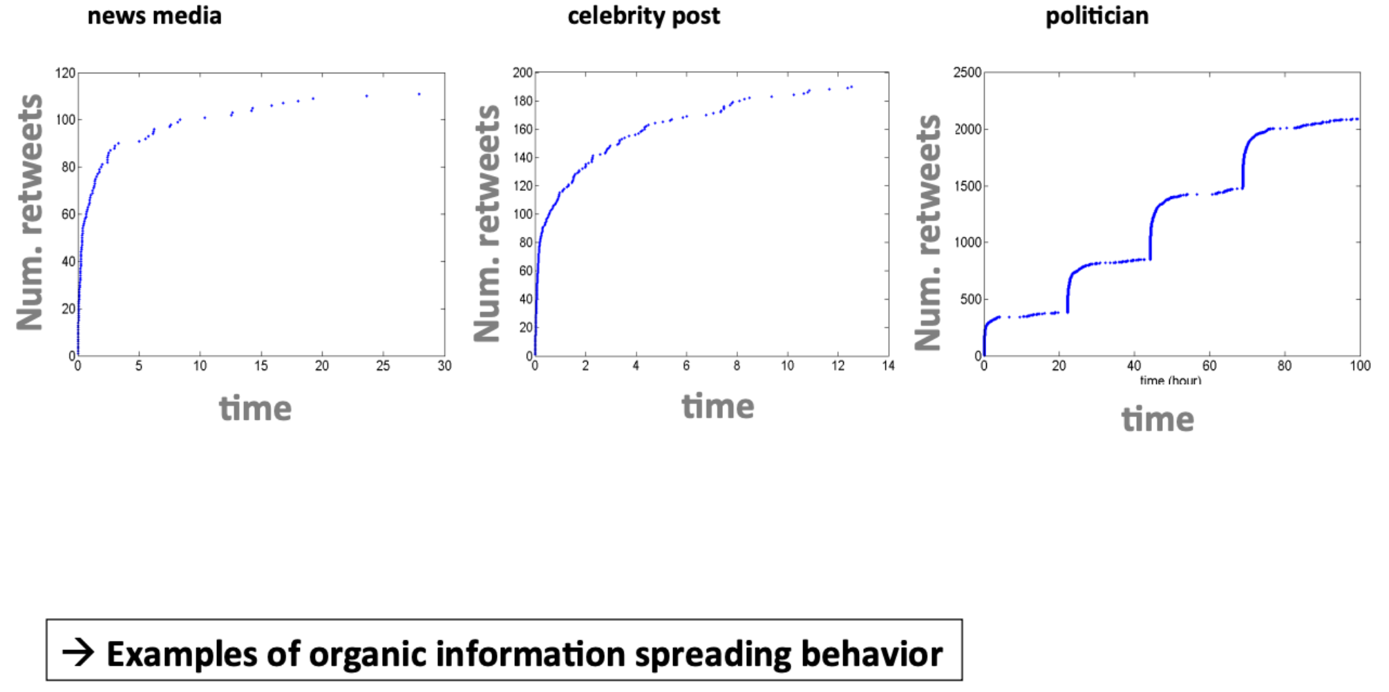
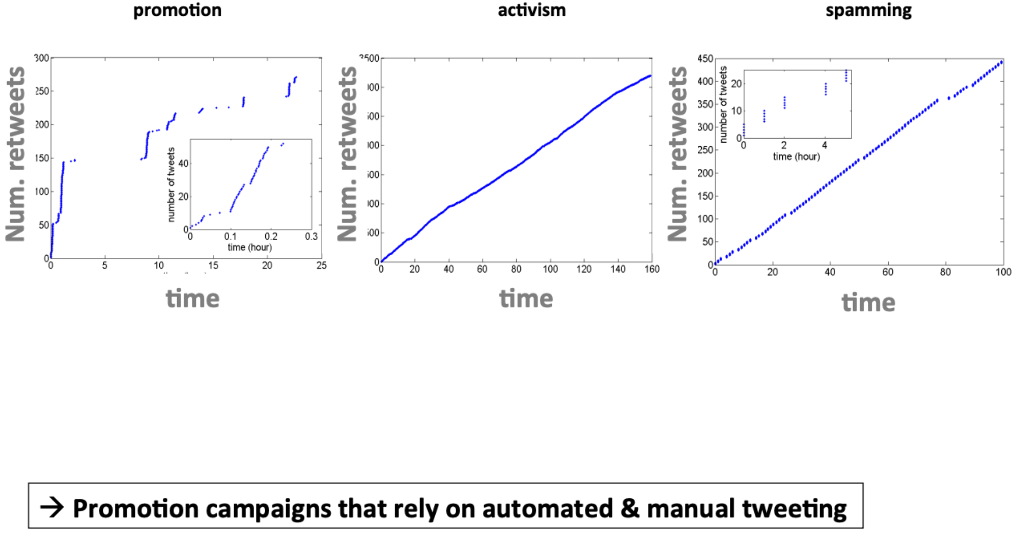
Characterizing activity: who tweets and when#

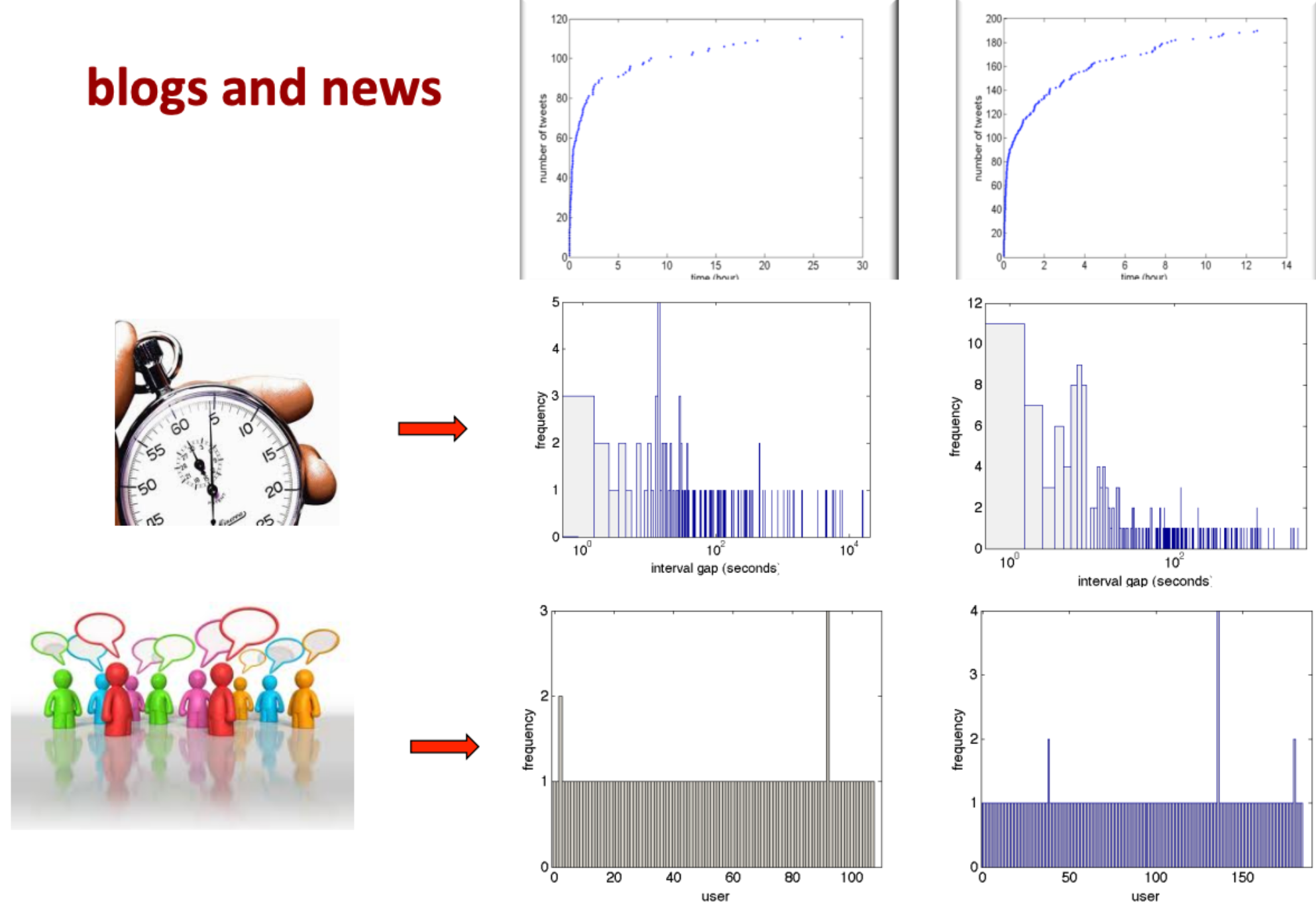
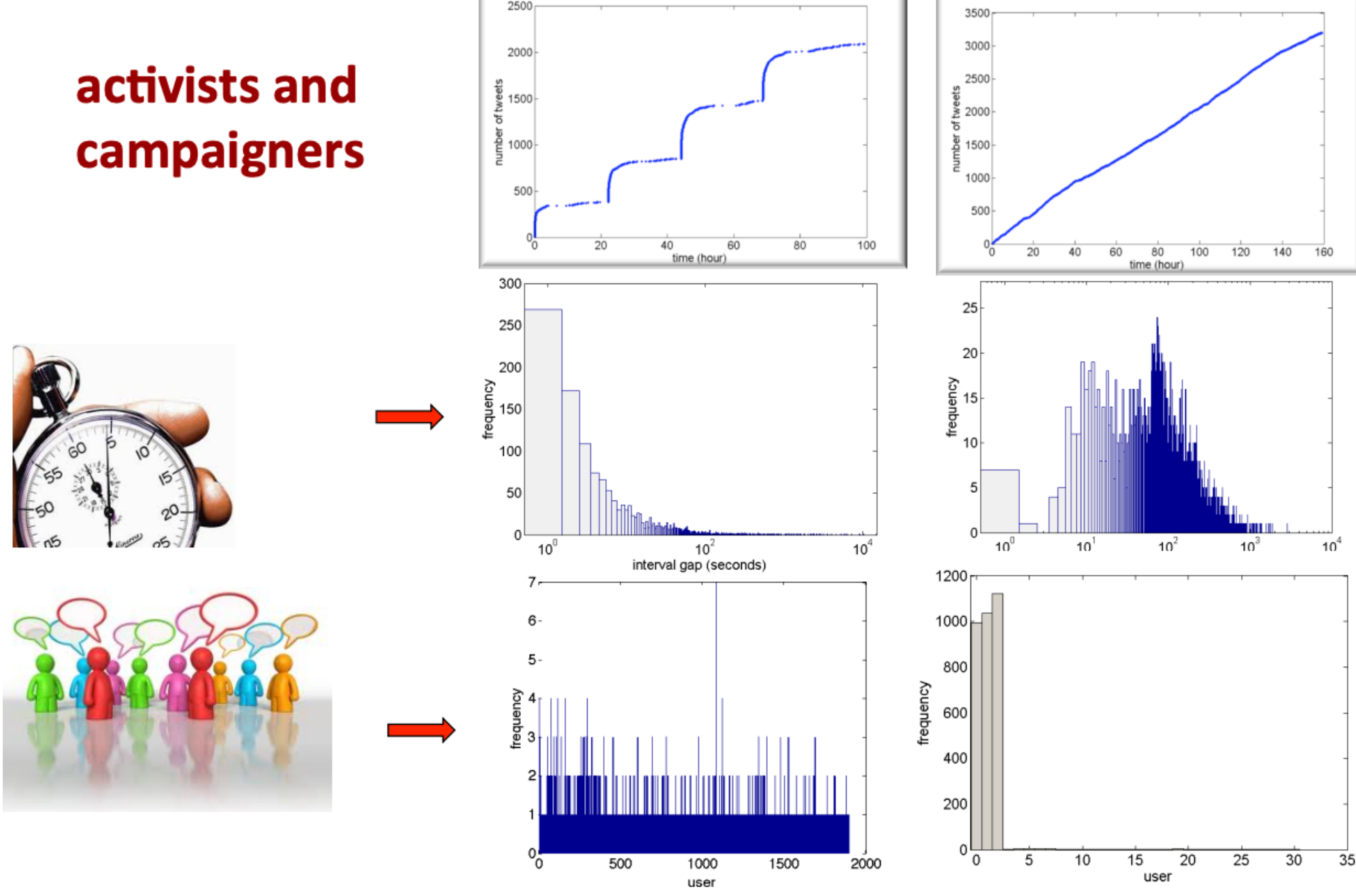
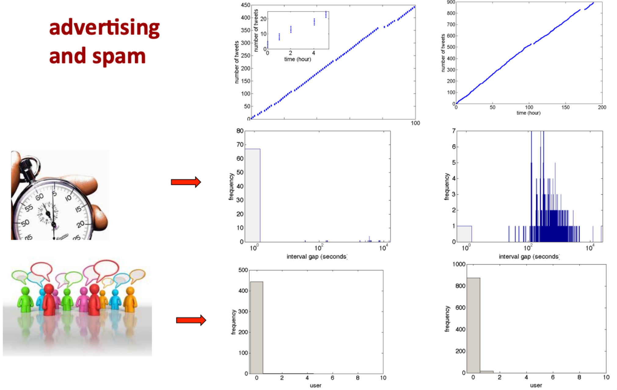
2 primary features found to be enough to classify Twitter behavior#

Characterizing user diversity#

The retweeting behavior among different users
This looks at the frequency counts as a function of user.

Characterizing time interval diversity#

The time in between retweeting from users (i.e., the regularity or predictability of the temporal trace of tweets)
This looks at the frequency of counts as a interval gap (in seconds).

Calculating user and time interval entropy#

\[ \text { entropy }=-\sum_{n=1}^{N} p\left(e_{n}\right) \ln p\left(e_{n}\right) \]

\[ p\left(e_{n}\right)=\frac{\text { freq }\left(e_{n}\right)}{\sum_{n=1}^{N} \text { freq }\left(e_{n}\right)} \]

For user entropy, $e_{n}$ is a specific user
For time interval entropy, $e_{n}$ is a unique interval (in sceonds)

User entropy#

Measures the number of times a specific user retweets some URL (specific tweet)
Random variable $F$ represents a distinct user in a trace $T_{j}$
Let there be $n_{f_{i}}$ retweets from user $f_{i}$ in the trace $T_{j}$
If $p_{F}$ denotes the probability mass function of $F$, such that $p_{F}\left(f_{i}\right)$ gives the probability of a retweet being generated by user $f_{i}$, then:

\[p_{F}\left(f_{i}\right)=\frac{n_{f_{i}}}{\sum_{k=1}^{n_{F}} n_{f_{k}}}\]

And user entropy $H_{F}$ is given by: $$ H_{F}\left(\mathcal{T}_{j}\right)=-\sum_{i=1}^{n_{F}} p_{F}\left(f_{i}\right) \log \left(p_{F}\left(f_{i}\right)\right) $$

Given the equation above, spam-like activity having small number of users responsible for large number of tweets, would have lower entropy than retweeting activity of news-worthy content

Time interval entropy#

Regularity or predictability of temporal trace of tweets
$\Delta T$ represents the time interval between 2 consecutives retweets in a trace $T_{j}$ (a tuple representing a user, whether they retweeted, and time)
$\Delta T$ has the possible values $\left\{\Delta t_{1}, \Delta t_{2}, \cdots, \Delta t_{i}, \cdots, \Delta t_{n_{T}}\right\}$
If there are $n_{\Delta t_{i}}$ time intervalsl of length $\Delta t_{i}$, then $p_{\Delta T}$ denotes the probability of observing a time interval $\Delta t_{i}$:

\[ p_{\Delta T}\left(\Delta t_{i}\right)=\frac{n_{\Delta t_{i}}}{\sum_{k=1}^{n_{T}} n_{\Delta t_{k}}} \]

Tweet activity in entropy plane#

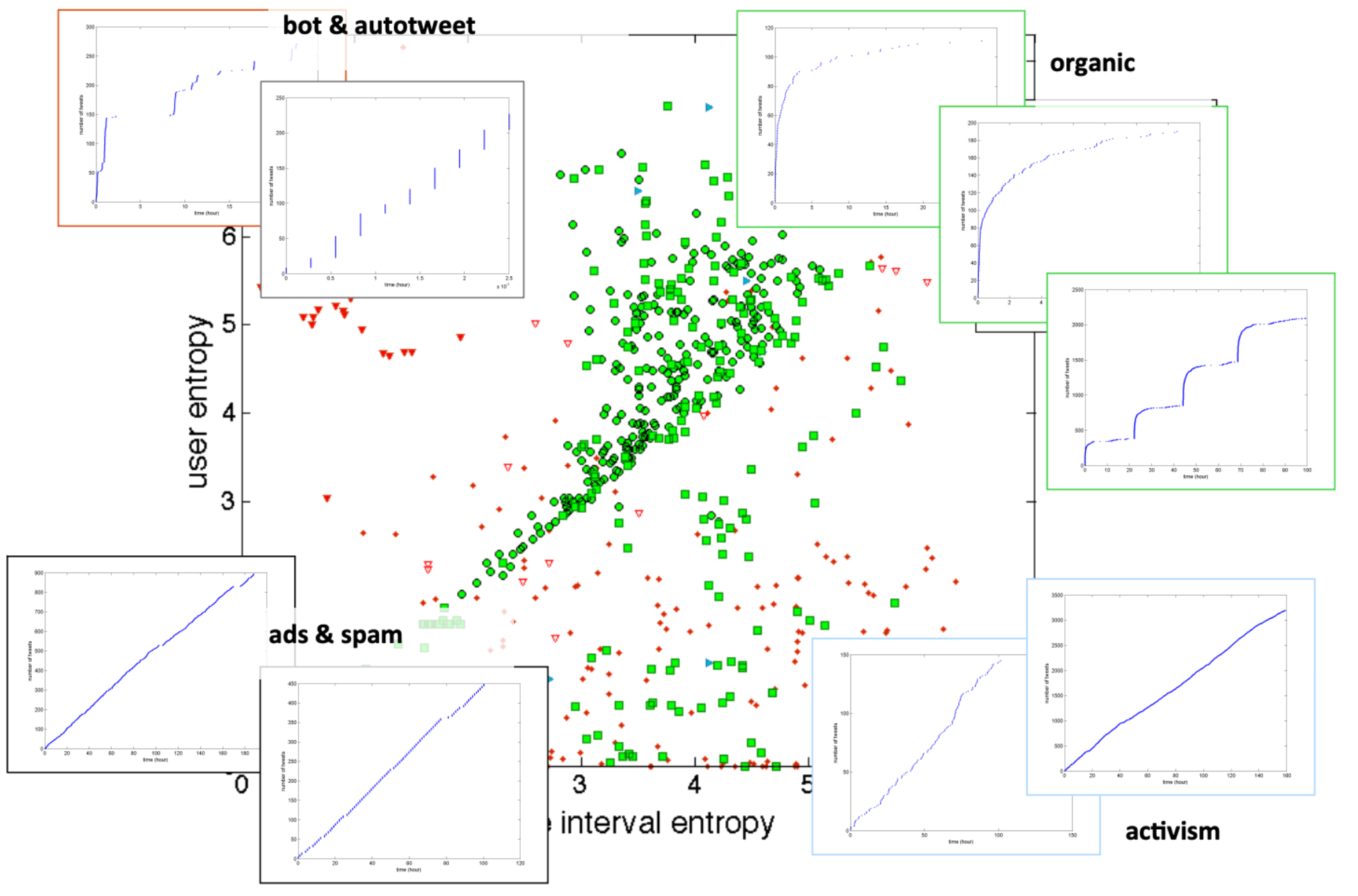
To interpret the above figure depicting different tweeting types in the entropy plane:

organic information spread: many individuals, many timescales
advertisements & promotions: few individuals, few timescales
campaigns: few individuals, many timescales
bot activity: many individuals, few time scales

Measuring influence via information transfer (transfer entropy) in social media (Ver Steeg & Galstyan, 2011)#

One important problem is the characterization and identification of influential individuals in social networks. These users are those who influence the behavior of large numbers of other users.
Prior work has used centrality measures such as PageRank (PR) to determine influential individuals. PR was invented by the founders of Google(!), and it evaluates the quality and quantity of links to a webpage to determine a relative score of that page’s importance authority on a 0 to 10 scale. Its key underlying assumption is that more important websites are likely to receive more links from other websites.
Additionally, websites that receive links from high PR websites will have higher PR than websites that have several but low PR websites linking to them.
This is because, to calculate PR for a given website, you take the sum of the PR of the linking websites (i.e., websites linking to the website you’re trying to calculate the PR for) and divide by the number of outgoing links from those websites.
For example, if you are trying to calculate the PR of website D, and website A has 1 outgoing link to D, you would calculate the PR of A and divide that by 1.

Ver Steeg & Galstyan point out, however, that this form of centrality may be misleading. PR is a topological centrality measure, which does not consider user dynamics. In other words, not all links in the above figure may actually be meaningful. High popularity does not necessarily equate to high influence.
- Semi-related to this point, in a paper from Banerjee et al., 2019, wherein 2 RCTs were performed to study gossip and information spreading, they took a similar perspective. Essentially, their goal was to transmit information as quickly and as widespread as possible within a village. Achieving this goal entails finding seeds or central nodes as they’re the optimal entrypoints for information diffusion (e.g., Gmail first invited leading bloggers to join and then added an ‘invite friends’ functionality). In this study, the researchers manipulated whether they spread information through village elders (high social status) or individuals that community members identified as best at spreading information (gossipers), likely due to how frequently they hear gossip that originated from that individual. Lo and behold, the latter was better at spreading information! (Truthfully, the definition of gossipers here feels circular to me, but I’m unsure how else one would define it.)

Influence via predictability#

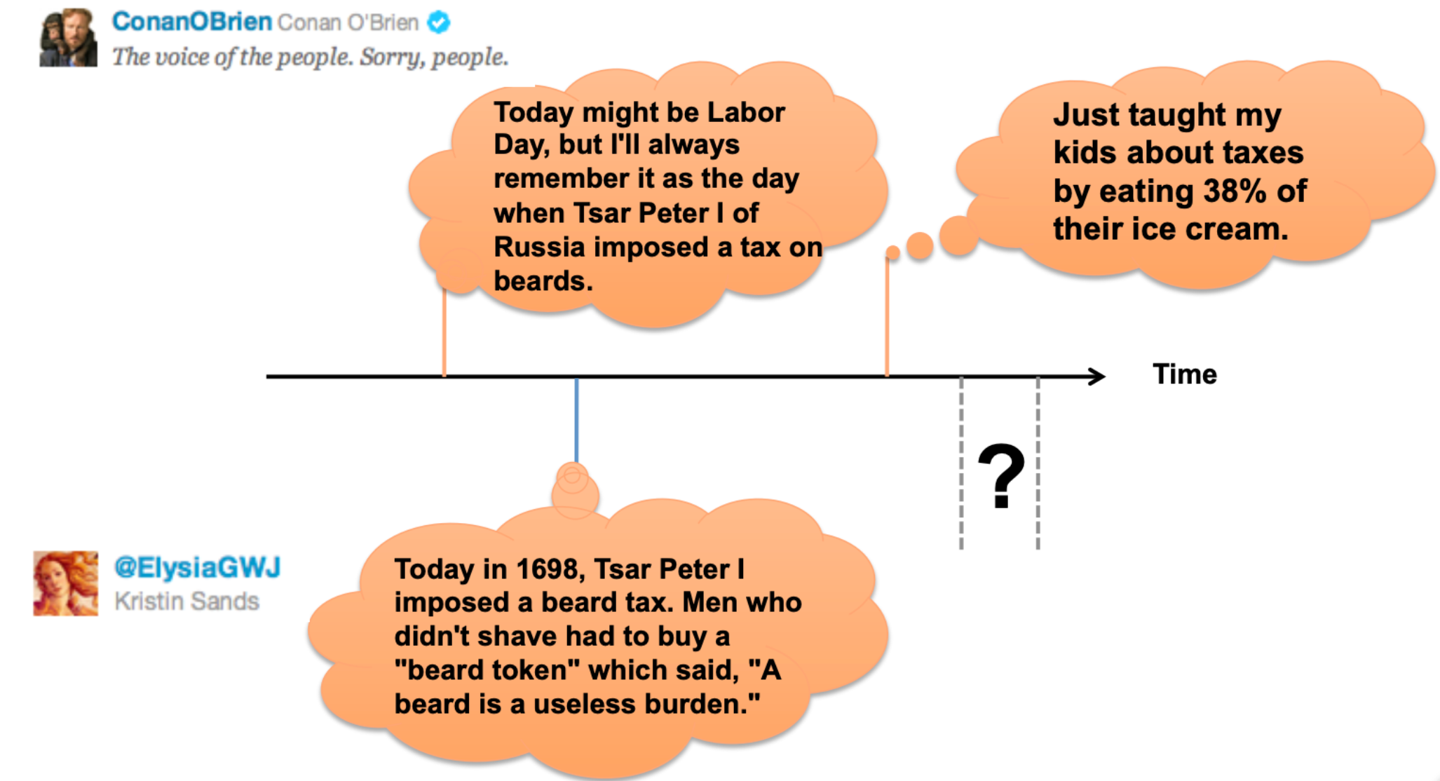
$Y$ influences $X$ if $Y$’s past activity is a good predictor of $X$’s future activity

You can quantify this type of influence using Transfer Entropy
- How much our uncertainty about user $X$’s future activity is reduced by knowing $Y$’s past activity!

Unlike correlation analyses like mutual information, transfer entropy allows us to look at directionality in the information flow, as it assumes some asymmetry.

Example:

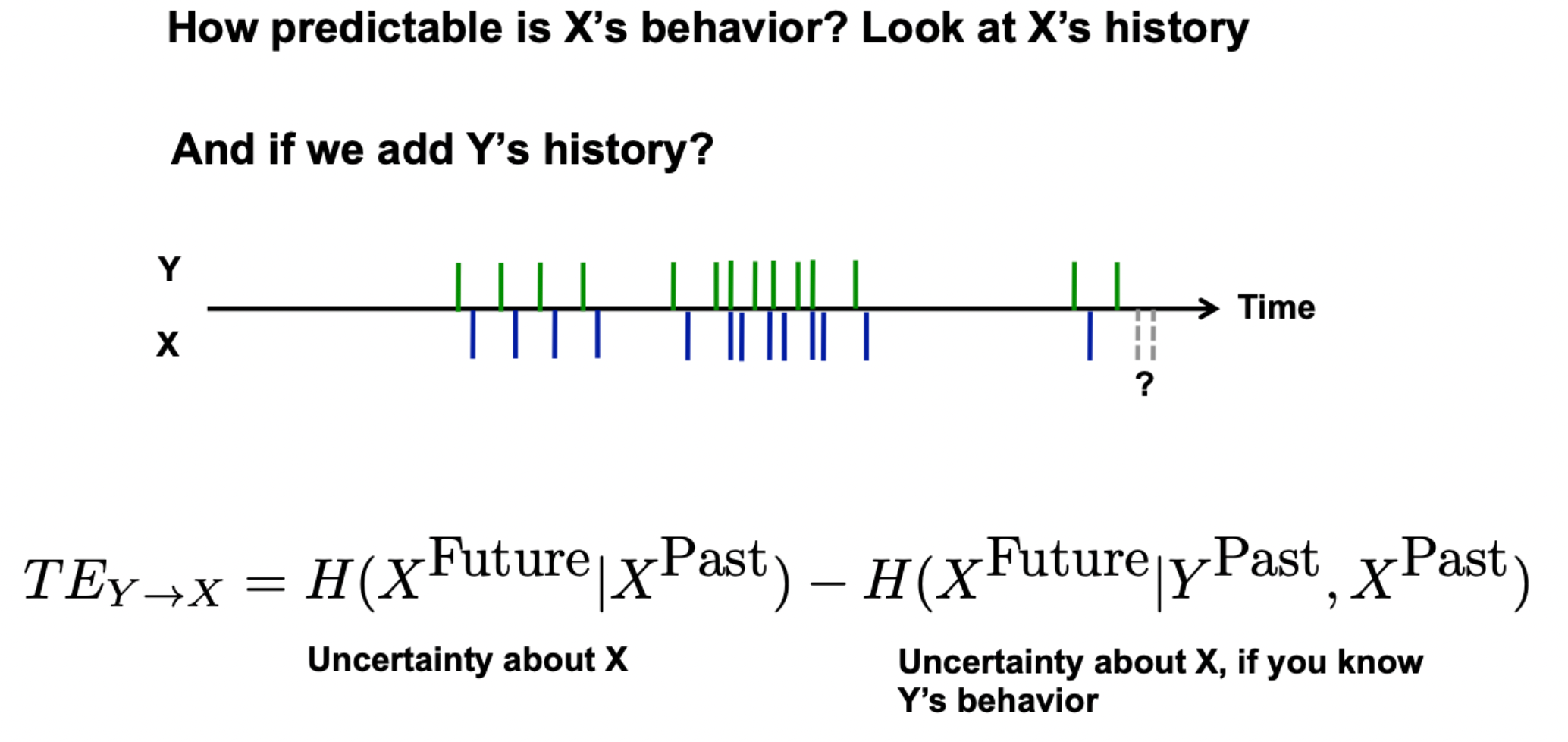
Hol’ up: Granger has some stuff to say (1969)#

This is a statistical hypothesis test that helps us determine whether one time series is useful in forecasting another time series.
Granger Causality: If a signal $Y$ “Granger-causes” (or “G-causes”) a signal $X$, then past values of $Y$ should contain information that helps predict $X$ above and beyond the information contained in past values of $X$ alone
- Assumes the cause happens before its effect
- Assumes the cause has unique information about the future value of its effect
- We don’t truly know if it’s the cause (hence, G-cause and not cause), but we do know that if it is a G-cause then it helps our prediction, and maybe that’s the next best thing when we don’t know the true cause.
A “Real World” example: if you’re trying to predict the price of houses in your area, you might want to know whether the house prices of a nearby area have any effect (or predict) on the house prices where you live. If they do, it’ll help you predict the house prices in your area.
To connect Granger Causality to neuroscience (from Wikipedia, kind of confuses me to be honest): if you want to predict how one neuron will fire (i.e., predict that neuron’s future), you can either use the entire neuronal ensemble or the entire ensemble subtracting out a certain target neuron. If the prediction is made worse by excluding the target neuron, then you can say it has a “g-causal” relationship with the current neuron.
Put another way, if you have 2 models describing the firing activity of both neurons $X$ and $Y$ over time, where model 1 is approximating activity of $X$ at a future timepoint to be the past activity of $X$, and model 2 is approximating $X$’s future activity as the sum of $X$ and $Y$’s past ctivity, then you can say that $Y$ is Granger-causal to $X$ if model 2 outperforms model 1.

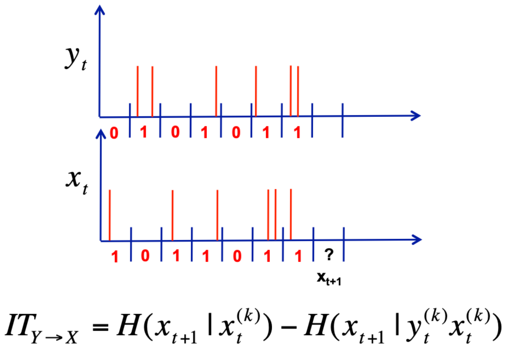
1 bit of information transfer from $Y$ to $X$ means we can use $Y$ to perfectly predict the next bit of $X$

So back to tweet timing and transfer entropy#

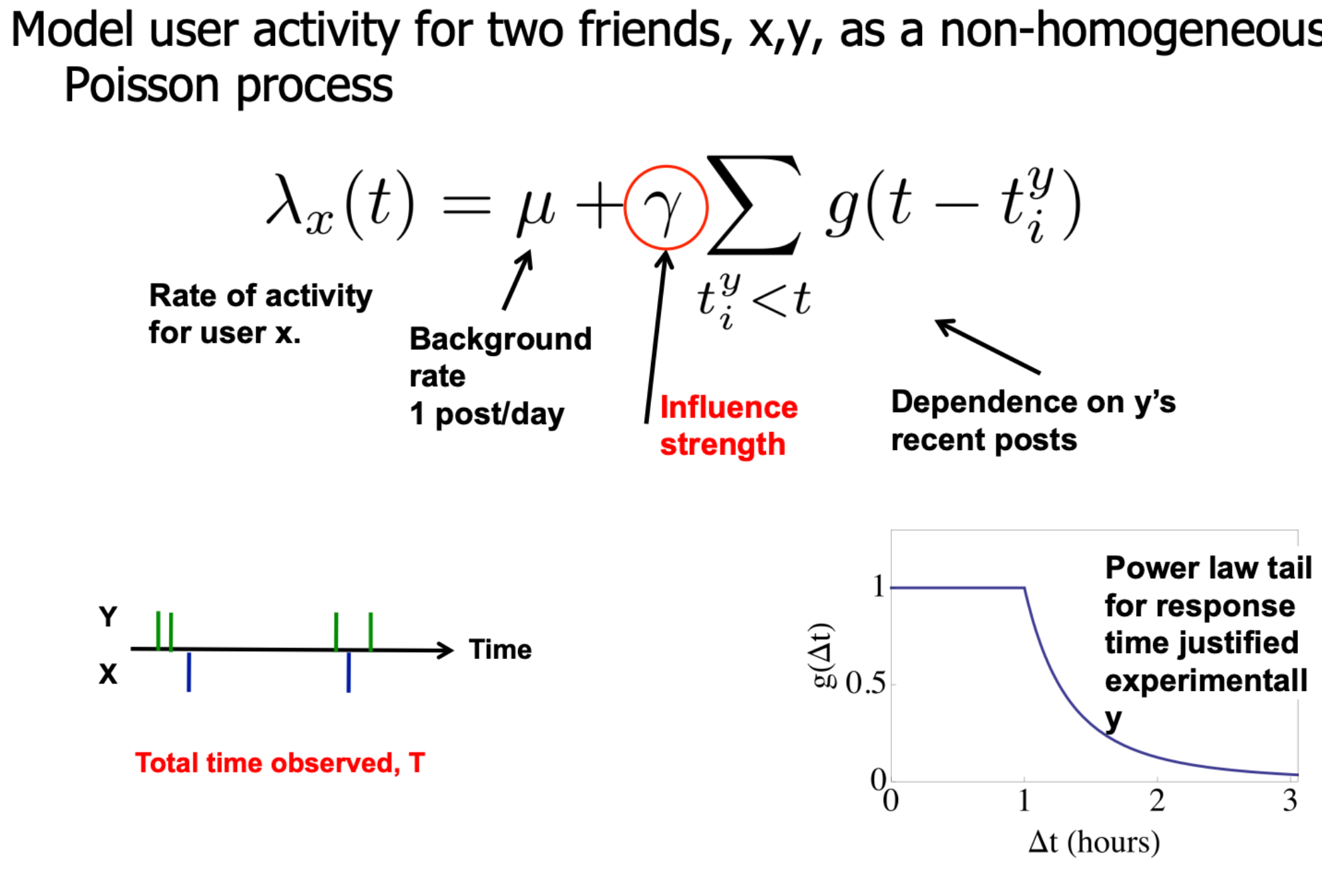
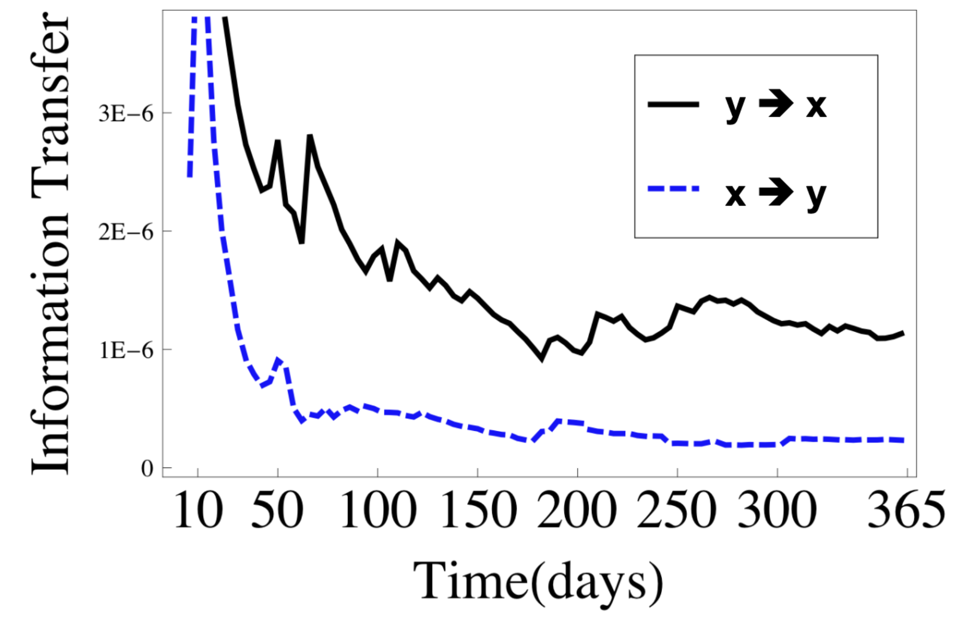
If $X$ is affected by $Y$, but not vice versa, this asymmetry can be captured using information transfer

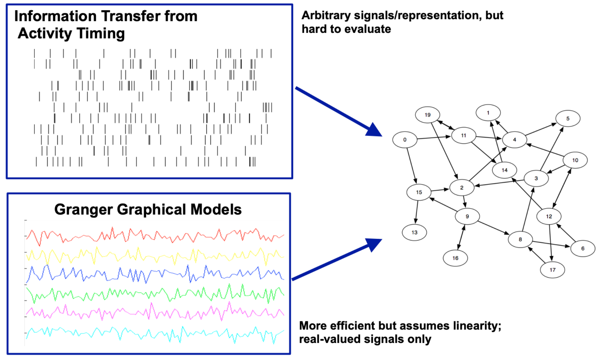
What if we had a whole raster plot (several users) and wanted to know who influences whom? And what if we wanted to recover the network?#

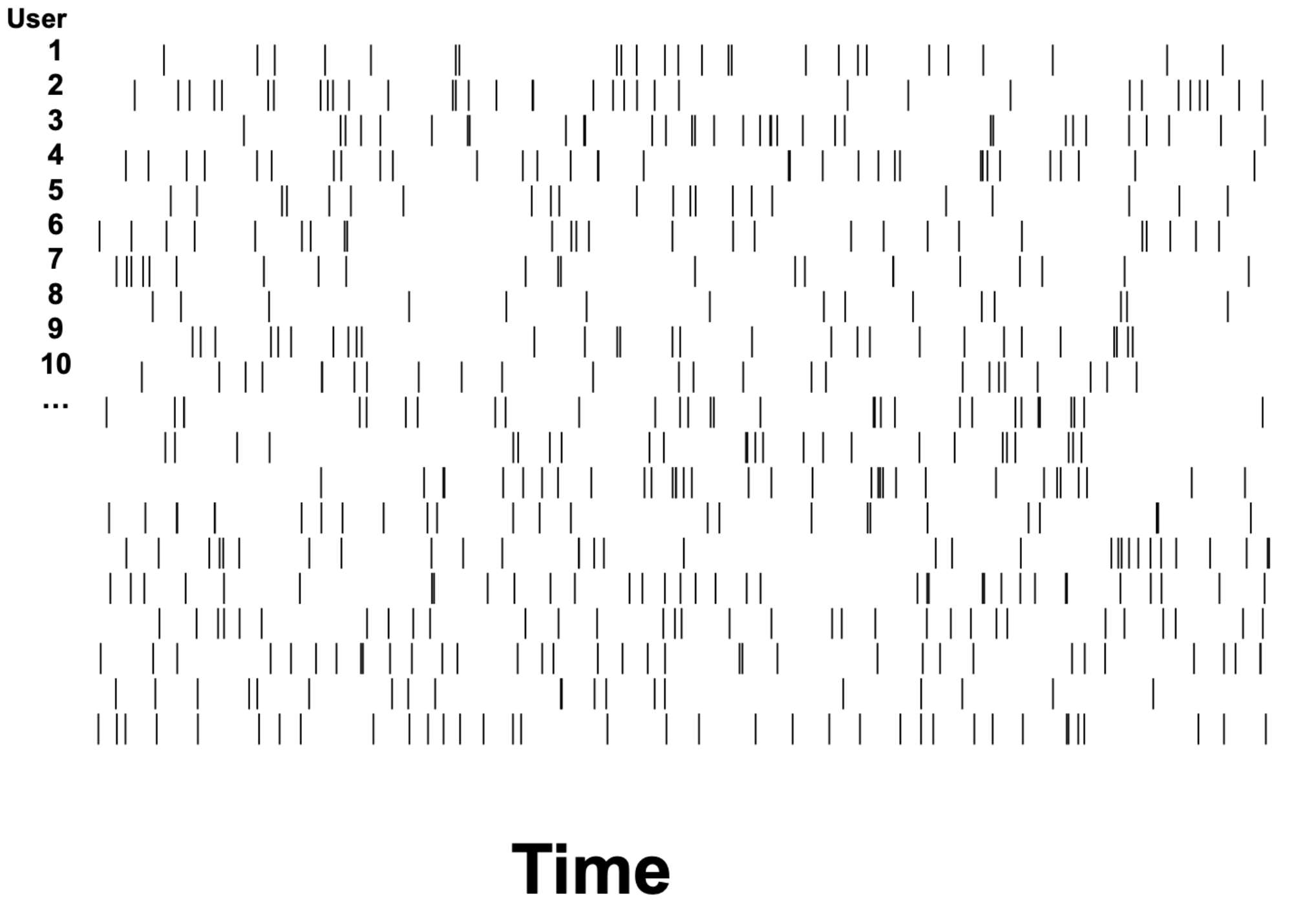
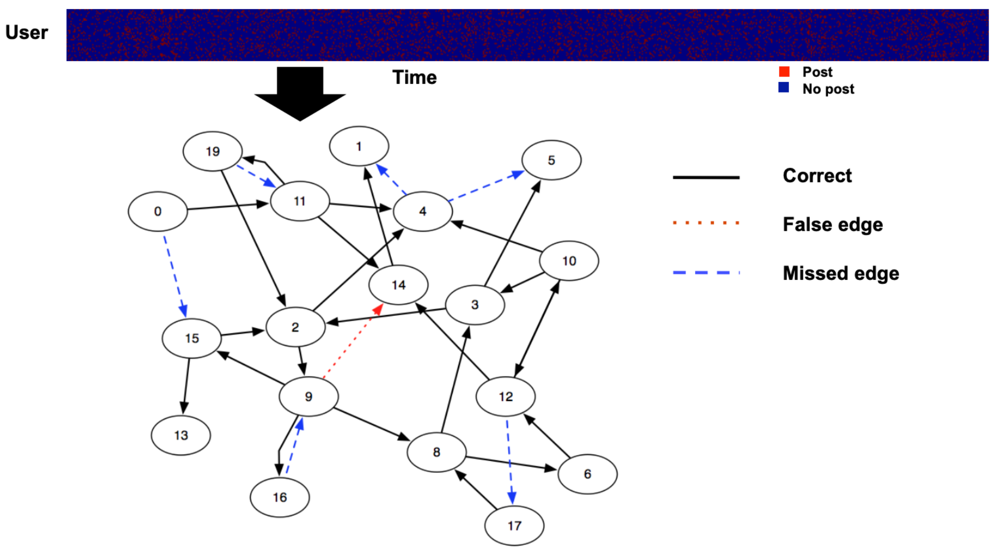
Ver Steeg & Galstyan, 2011 found that ~50 posts/person typically leads to perfect reconstruction of the network.

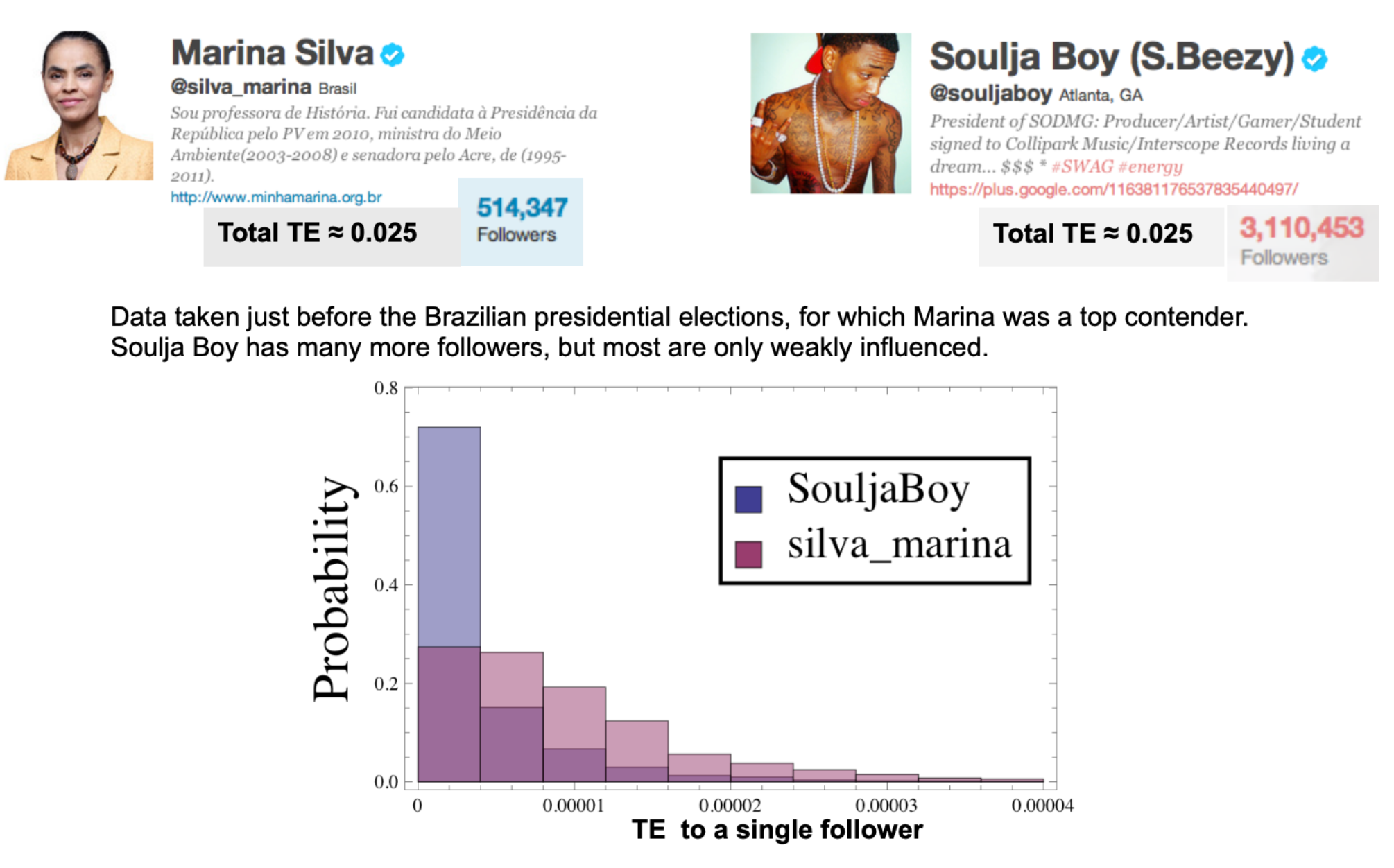
Example of 2 users with the same TE#

Now return to Granger Causality#

Twitter time series could be # of tweets by a user in a given timeframe (e.g., tweets per day) or # of hashtags, etc.
What if we wanted to calculate an influence network using Granger Causality?
- Calculate all possible pair-wise influence between every possible time series pairing
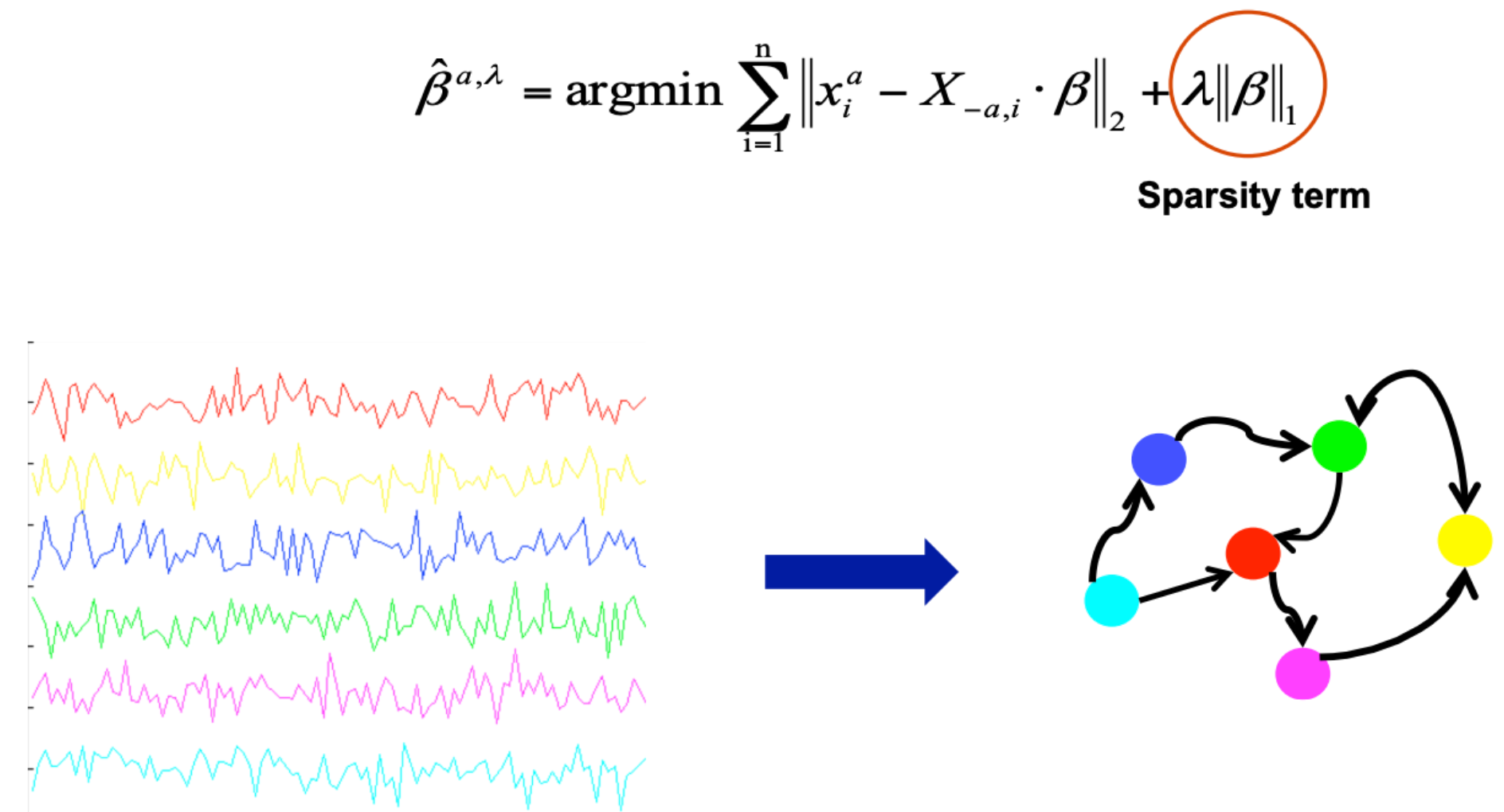
HOWEVER, PROBLEM: The learned influence network will be generally very dense
Solution: You can magically add a sparsity term:

Summary#

Transfer entropy: how much is our uncertainty about user $X$’s future activity reduced by knowing about $Y$’s past activity?
Granger Causality: $Y$ is “Granger-causal” to $X$ if the model summing the past activity of both $X$ and $Y$ is a better predictor of $X$’s future activity than $X$’s past activity alone.